Circuit Switching Routing

In the previous cases we assumed that PEs receive data in full for itself and all its successors. Then, the part of the load is sent to the idle neighbors. This is a feature of the so-called store and forward routing. There exists a different routing strategy called circuit switching. In circuit switching a direct (electrical) connection between the sender and the receiver is established. Consequently, the communication delay does not depend significantly on the covered distance. Hence, it can be advantageous to send some data far ahead and then redistribute it from two (or more) points. A similar situation takes place for some packet-switching communication methods (e.g. wormhole routing) [NMK93]. 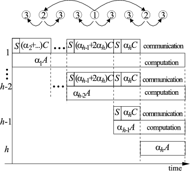In the following we assume that the originator is located in the center of the linear array network, results are not returned, all PEs have network processors and can simultaneously transmit over both ports. The originator sends data simultaneously to two distant PEs. In the next step both the originator and the two previously activated PEs send data to two new processors (cf. Fig.2). The process is repeated activating in each step twice as many processors as were active at the beginning of the step. We will call by a layer the set of PEs activated in the same distribution step. Thus, all processors are working after $h\!=\!\lceil\log_3m\rceil$ steps.

Figure 2: Communication and computation in a linear array with circuit-switching routing.

Distributing data and a diagram of communication and computing is depicted in Fig. 2. We denote by $A$ the processing rate of all (identical) processors, by $C$ the communication rate of all links, by $S$ the startup time of all links, by $h$ the number of steps in data distribution algorithm, and by $\alpha_i$ the load of each PE in layer $i$. Since no results are returned, all the PEs must finish their computations simultaneously. Note that the time of computing on the PEs of the sending layer is equal to the time of communicating to and computing on the PEs of the receiving layer (cf. Fig. 2). Thus, equations (1) have now the form:

$$\alpha_{h-i}A\!\!\!\! = S\!+\!(\alpha_{h-i+1}\!+%% \!2\!\sum_{j=2}^i3^{j-2}\alpha_{h-i+j})C\!+\!\alpha_{h-i+1}A,\,\,\,\, i\!=\!1,\dots,h\!-\!1$$

$$V = \alpha_1+2\sum_{j=2}^h3^{j-2}\alpha_j$$ (4)

The above set of equations can be solved in $O(h)=O(\log\,m)$ time by a method analogous to the one proposed to solve equations (1).