Basic Model

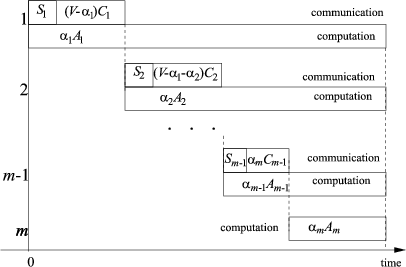
We will describe now a basic model for the linear array network. A Gantt chart of communications and computations is depicted in Fig. 1.

Figure 1: Communication and computation in a linear array of processors.

For simplicity of the presentation we assume first that no results are returned to the originator, the PEs have network processors and the originator is located at the end of the chain. The part of the load which is not processed by the originator is sent to the nearest neighbor. The neighbor divides the received data into a part processed locally and forwards the rest to the next idle processor. This procedure is repeated until the last processor is activated. Since there is no returning of data all the processors must stop computing at the same moment of time [BD97,CR88]. As can be observed in Fig.1, processing on a sending PE lasts as long as communication to the receiver and processing on the receiver. Thus, we can find a distribution of the load from the following set of equations [BD97,CR88]:

$$\alpha_iA_i = S_i+(\alpha_{i+1}+\dots+\alpha_m)C_i+\alpha_{i+1}A_{i+1}, {\rm\hspace{1.5mm}} i=1,\dots,m-1$$

$$V = \alpha_1+\alpha_2+\dots+\alpha_m$$ (1)

$$\alpha_1,\alpha_2,\dots,\alpha_m\geq 0$$

where $S_i, C_i$ are startup time and transmission rate of a link joining $P_i$ and $P_{i+1}$, and $A_i$ is processing rate of $P_i$. The above equation set can be solved in $O(m)$ time by a reduction of $\alpha_i$ to a linear function of $\alpha_m$: $\alpha_{i}=k_i\alpha_m+l_i$, where $k_{m}=1, l_m=0, k_{i}=\frac{C_i}{A_{i}}\sum_{j=i+1}^{m}k_i+\frac{A_{i+1}}{A_i}k... ...\frac{C_i}{A_{i}}\sum_{j=i+1}^{m}l_i+\frac{A_{i+1}}{A_i}l_{i+1}+\frac{S_i}{A_i}$ for $i=1,\dots,m-1$. From the last equation of formulation (1) we obtain $\alpha_m=(V-\sum_{i=1}^ml_i)(\sum_{i=1}^mk_i)$. It may happen that a feasible solution of equations (1) does not exist. Practically spoken, it means that data can be processed by less than $m$ processors in a shorter time than required to activate all $m$ PEs. Then, the maximum number of usable processors and the optimal distribution of the load can be found by a binary search over $m$ in time $O(m\log m)$.