A ![]() -dimensional hypercube network consists of
-dimensional hypercube network consists of ![]() PEs.
Each of the PEs can be labeled by a unique
PEs.
Each of the PEs can be labeled by a unique ![]() -bit
binary word such that directly connected processors
have their labels differing in exactly one bit.
The idea of divisible task was applied to hypercubes in [BD95,BD97].
The scattering method was based on consecutively
activating the nearest neighbors of the active processors.
Thus, the originator
-bit
binary word such that directly connected processors
have their labels differing in exactly one bit.
The idea of divisible task was applied to hypercubes in [BD95,BD97].
The scattering method was based on consecutively
activating the nearest neighbors of the active processors.
Thus, the originator ![]() (labeled (0,...,0)) activated
(labeled (0,...,0)) activated ![]() PEs
with exactly one 1 in the label.
Those PEs, in turn, activated PEs with exactly two 1's in the label etc.
Let us call by a layer the set of PEs activated in the same step
of scattering, i.e. the set of PEs with the same number of
1's in their labels.
Note that each PE in layer
PEs
with exactly one 1 in the label.
Those PEs, in turn, activated PEs with exactly two 1's in the label etc.
Let us call by a layer the set of PEs activated in the same step
of scattering, i.e. the set of PEs with the same number of
1's in their labels.
Note that each PE in layer ![]() can be reached
by
can be reached
by ![]() links (the number of 1's in the label), and has
links (the number of 1's in the label), and has
![]() inactive neighbors in layer
inactive neighbors in layer ![]() .
The number of PEs in layer
.
The number of PEs in layer ![]() is
is
![]() .
We assume that PEs are identical, each PE has a network processor and
the time of returning the results is negligible.
Then, the diagram of computing and communication is the same as
the one in Fig.1, and processors of the layer
activated earlier compute as long as it is required to
send data to the next layer and compute on the next layer.
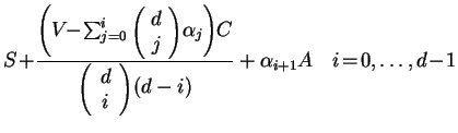
Thus, distribution of the load can be found from
the following equations:
.
We assume that PEs are identical, each PE has a network processor and
the time of returning the results is negligible.
Then, the diagram of computing and communication is the same as
the one in Fig.1, and processors of the layer
activated earlier compute as long as it is required to
send data to the next layer and compute on the next layer.
Thus, distribution of the load can be found from
the following equations: