Performance Prediction Based on the Divisible Task Model - example

In this section we give some examples of applying the divisible task method. First let us consider a numerical example.

Consider a computer system consisting of four identical PEs connected by identical communication links. Each PE has a network processor, and is capable of simultaneous computing and communicating. The amount of the returned results is constant and equal to 1024 bytes. The order of data return is the order of activating PEs (cf. Fig.4(b)). We use equations (7) to find the distribution of the load. From the solution one can compute the total processing time, which is $A\alpha_1$. In the following table results of solving equations (7) for $m=4, V=10^6$ bytes, are presented.

	system A	system B	system C
$A$[s/byte]	0.0002324	0.000692	0.000596
$C$[s/byte]	1E-11	1.25E-08	1.7485E-06
$S$[s]	1.08E-07	3.9E-05	0.0011377
processing time [s]	581	1730	1497

In the above table parameters $A, S, C$ were not intended to represent any particular computer system. Still, system A may represent a shared memory supercomputer from the 80-ties, system B is a representative of massively parallel message passing computer from the beginning of the 90-ties, while system C is a cluster of contemporary (1997) PC-compatible computers with Linux operating system and PVM. The conclusion that can be derived from the above table is that contemporary PCs are as good as leading computers 6-7 years ago. Thus, time beats any machine.

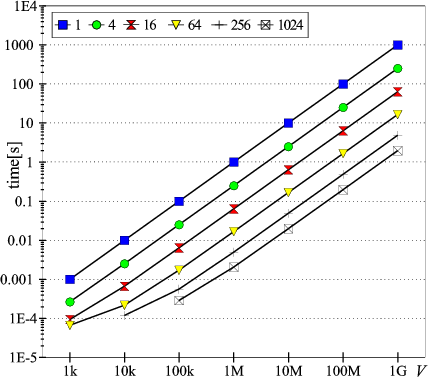
As we are able to compute the processing time for the whole load both on a single machine, and on the given number of PEs, we are also able to compute speedup, utilization etc. for the considered computer system and communication algorithm. In the following example we will analyze a 3-dimensional mesh with PEs using 1 port at a time ($p=1$) and circuit switched routing. Since speedup can be an ambiguous performance measure, we will concentrate on the processing time. In Figs.6 and 7 we present a relation between the processing time and the volume of work $V$ for 1-, 4-, 16-, 64-, 256-, 1024-processor systems. In both figures the communication parameters are $C=10^{-9}\frac{s}{byte}$, and $S=10^{-5}s$. In Fig.6 processors have $A=10^{-6}\frac{s}{byte}$, and in Fig.7 processing rate is better and equal to $A=10^{-8}\frac{s}{byte}$.

Figure 7: Processing time in a 3-dimensional mesh of PEs vs. volume of work, and processor number for $A=10^{-6}\frac{s}{byte}$.

Figure 8: Processing time in a 3-dimensional mesh of PEs vs. volume of work, and processor number for $A=10^{-8}\frac{s}{byte}$.

As it can be seen in both figures not all volumes can be processed by any number of processors. Communication time dominates in the processing time when the volume is small. Therefore, only few processors can be activated before completing the task. When $V$ is big, the dependence of processing time on $m$ and $V$ is close to linear. In the system with faster processors bigger loads are needed to activate all PEs. The curves for $m=64,\dots,1024$ are hardly distinguishable in Fig.7. This means that increasing the number of processors gives a diminishing decrease in processing time. Furthermore, the decrease is worse in faster systems. A similar effect can be observed for worse communication parameters $C,S$ at constant processing rate $A$. We can conclude from this comparison, that the relentless progress in processor speed must be matched by an equal advancement of the communication systems. Otherwise parallel computers, sooner or later, will be outperformed by single-processor machines.