In a regular non-toroidal ![]() -dimensional mesh each PE is directly
coupled up to
-dimensional mesh each PE is directly
coupled up to ![]() neighbors (cf. Fig.5).
In the toroidal mesh PEs at the mesh opposite 'sides' are connected,
and each PE is connected with exactly
neighbors (cf. Fig.5).
In the toroidal mesh PEs at the mesh opposite 'sides' are connected,
and each PE is connected with exactly ![]() neighbors.
We assume here that communication links and processors are identical,
PEs are equipped with network processors,
results are not returned to the originator located
in the center of the network.
Each PE is capable of simultaneous communication over
neighbors.
We assume here that communication links and processors are identical,
PEs are equipped with network processors,
results are not returned to the originator located
in the center of the network.
Each PE is capable of simultaneous communication over
![]() links (ports).
We will call by a layer the set of PEs
activated in the same stage of data distribution.
links (ports).
We will call by a layer the set of PEs
activated in the same stage of data distribution.
Two-dimensional rectangular mesh networks with store-and-forward
communication mode were considered in [BD96].
A scattering method based on routing messages
only between the nearest neighbors was presented.
Thus, the layers of PEs form squares around the originator.
In [BDGT99] a more efficient method based on circuit-switched routing
was proposed for a two-dimensional mesh.
Scattering methods were further extended in [D97] to the case
of a 3-dimensional mesh with ![]() .
Due to space limitations we describe only the case of
.
Due to space limitations we describe only the case of ![]() in 3-dimensional mesh (the following discussion
and formulae apply also in the case of
in 3-dimensional mesh (the following discussion
and formulae apply also in the case of ![]() ).
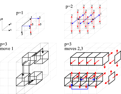
The methods of scattering in 3-dimensional mesh
for PEs using
).
The methods of scattering in 3-dimensional mesh
for PEs using ![]() ports simultaneously are depicted
in Fig.5.
ports simultaneously are depicted
in Fig.5.
The algorithms are based on recursive division
of the mesh into sub-meshes of smaller size.
In each step of scattering ![]() PEs are activated.
These PEs become originators for scattering in the next step.
Thus, in each step the initial mesh is divided into
PEs are activated.
These PEs become originators for scattering in the next step.
Thus, in each step the initial mesh is divided into ![]() submeshes of
submeshes of ![]() times smaller size.
Each of the steps consists, in turn, of three moves.
The same moves are performed simultaneously by all the active PEs.
Each move increases the number of active PEs
times smaller size.
Each of the steps consists, in turn, of three moves.
The same moves are performed simultaneously by all the active PEs.
Each move increases the number of active PEs ![]() times,
which is maximum because only
times,
which is maximum because only ![]() ports can be used simultaneously.
Hence, after
ports can be used simultaneously.
Hence, after ![]() moves the number of working PEs is
moves the number of working PEs is ![]() .
For
.
For ![]() and
and ![]() , each move of a step activates
, each move of a step activates ![]() PEs neighboring along a different dimension.
In a 3-port system the originator activates three PEs
located in the same two-dimensional cross-section
of the initial mesh (say, along the plane
PEs neighboring along a different dimension.
In a 3-port system the originator activates three PEs
located in the same two-dimensional cross-section
of the initial mesh (say, along the plane ![]() ).
Next, the four active PEs send data along the third dimension
(
).
Next, the four active PEs send data along the third dimension
(![]() dimension).
In the third move each active processor sends data
to the neighbors along the hull of the initial mesh and to one
neighbor inside the mesh.
dimension).
In the third move each active processor sends data
to the neighbors along the hull of the initial mesh and to one
neighbor inside the mesh.
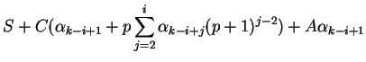
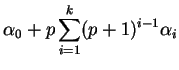
Let us denote by ![]() the amount of data to be processed
by a PE activated in move
the amount of data to be processed
by a PE activated in move ![]() ,
and by
,
and by ![]() the number of moves.
The diagram of communication and computation is given
in Fig.2, but here the number of
ports involved simultaneously can be greater.
Similarly, computing on the sending layer of PEs lasts as long as
communicating to and computing on the PEs of the receiving layer.
The distribution of data can be found from the following set of equations
(
the number of moves.
The diagram of communication and computation is given
in Fig.2, but here the number of
ports involved simultaneously can be greater.
Similarly, computing on the sending layer of PEs lasts as long as
communicating to and computing on the PEs of the receiving layer.
The distribution of data can be found from the following set of equations
(
![]() ):
):
A broadcasting method for ![]() -dimensional toroidal mesh with
-dimensional toroidal mesh with
![]() -port PEs and edge size
-port PEs and edge size ![]() (
(![]() ) has been proposed
in [PC96].
This method activates
) has been proposed
in [PC96].
This method activates ![]() PEs in
PEs in ![]() moves.
Thus, the methods proposed here can be extended to toroidal meshes
of arbitrary dimension when
moves.
Thus, the methods proposed here can be extended to toroidal meshes
of arbitrary dimension when ![]() .
Observe that also scattering methods for
.
Observe that also scattering methods for ![]() and
and ![]() can be
applied in meshes of higher dimension.
The proposed scattering algorithms are optimal in the sense that
the number of activated processors in the allowed number of steps
is the biggest possible.
Equations (10) can be applied in any
architecture in which PEs can be activated in the same way as above,
i.e. each active PE in each move starts
can be
applied in meshes of higher dimension.
The proposed scattering algorithms are optimal in the sense that
the number of activated processors in the allowed number of steps
is the biggest possible.
Equations (10) can be applied in any
architecture in which PEs can be activated in the same way as above,
i.e. each active PE in each move starts ![]() new processors.
One of such architectures can be multistage interconnection
[D97].
new processors.
One of such architectures can be multistage interconnection
[D97].