Krzysztof Krawiec
Segmenting Retinal Blood Vessels with Deep Neural Networks
This page contains the material accompanying the paper accepted for publication in IEEE Transactions on Medical Imaging: Segmenting Retinal Blood Vessels with Deep Neural Networks by Paweł Liskowski and Krzysztof Krawiec.
@ARTICLE{7440871,
author={P. Liskowski and K. Krawiec},
journal={IEEE Transactions on Medical Imaging},
title={Segmenting Retinal Blood Vessels with Deep Neural Networks},
year={2016},
volume={PP},
number={99},
pages={1-1},
keywords={Biomedical imaging;Blood vessels;Convolution;Databases;Image segmentation;
Neural networks;Pathology;Classification;deep learning;neural networks},
doi={10.1109/TMI.2016.2546227},
ISSN={0278-0062},
month={},}
New: Segmentations produced by the networks trained on all image patches
We trained and tested a few networks on all patches, i.e., also those that extend beyond the FOVs (and thus contain some black background from beyond the FOVs. The visualizations can be downloaded here:
- For the test set of the DRIVE database: structured prediction
- For the STARE database: structured prediction
Segmentations for all images
The ZIP archives linked below contain the outputs produced by the NO-POOL-SP neural network, the one that achieved the best overall results in the paper. Each archive contains PNG/JPG files for each fundus image for all three databases we used in the paper. We provide two sets of files: raw (direct output of the neural network, which has the interpretation of probability) and binarized (network output thresholded at 0.5).
- For DRIVE database: raw and binarized,
- For STARE database: raw and binarized,
- For CHASE database: raw and binarized.
Our networks are trained and tested only on the 27x27 patches that fit entirely within the field of view (FOV). FOVs are given for the DRIVE database, and for the STARE database we calculate them from images using the ImageJ script below. Click here to download a zipped directory structure with B&W images defining the pixels (together with the surrounding 27x27 patches) on which our networks were trained and tested.
ImageJ script
Click here to open the ImageJ script for partitioning the manual segmentations into capillaries and thick vessels in Section VIII (JavaScript file, renamed to *txt due to security requirements).
Figures from the paper
Fig. 1 A training image from the DRIVE database (left) and the corresponding manual segmentation (right).
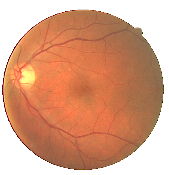
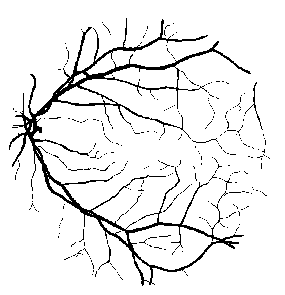
Fig. 2 A pathological image from the STARE database (left) and the corresponding manual segmentation (right).
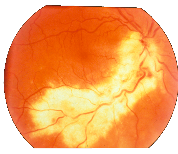
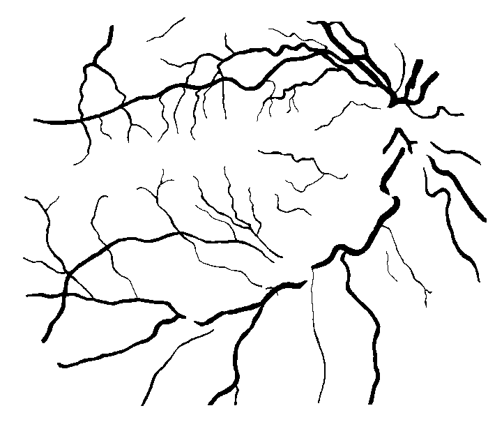
Fig. 3 Architecture of a convolutional neural network with three convolutional layers, one pooling layer, and two fully-connected layers. The network uses 3x3 convolution units with stride 1 and 2x2 pooling units with stride 2.
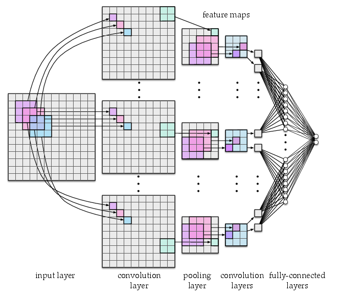
Fig. 4 Examples of positive (left) and negative (right) 27x27 training patches extracted from the DRIVE images.
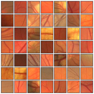
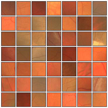
Fig. 5 Examples of positive (left) and negative (right) training patches after applying GCN transformation.
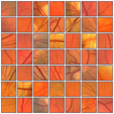
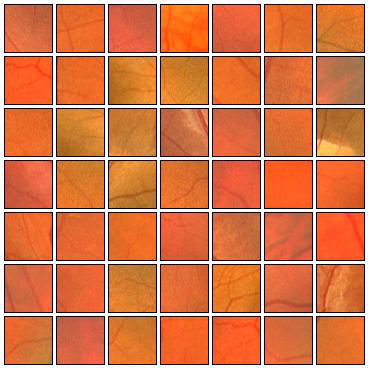
Fig. 6 Positive (left) and negative (right) training patches after applying ZCA whitening transformation.
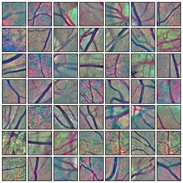
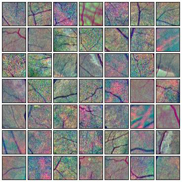
Fig. 7 Augmentations of positive (left) and negative (right) training patches. Each row shows 6 random augmentations of the leftmost patch.
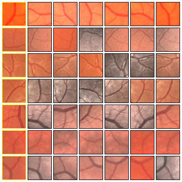
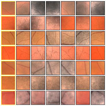
Figure 8: A training example for the SP approach: the 27×27 patch with the s × s = 5 × 5 output window (left) and the corresponding desired output (right).
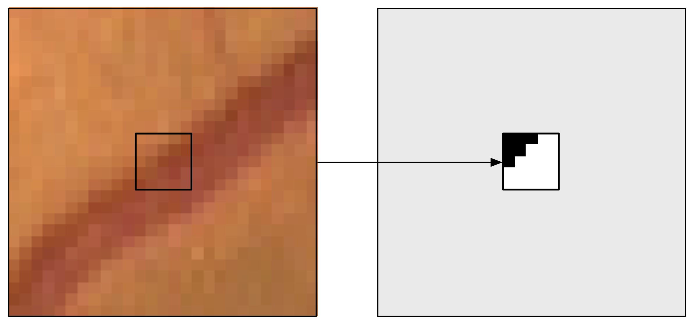
Figure 9: Ground truth (left) and segmentation result (right) for two healthy subjects: (a) DRIVE image #13, (c) STARE image #0255, and two subjects with pathologies: (b) DRIVE image #8, (d) STARE image #0002.
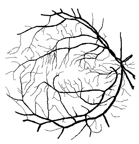

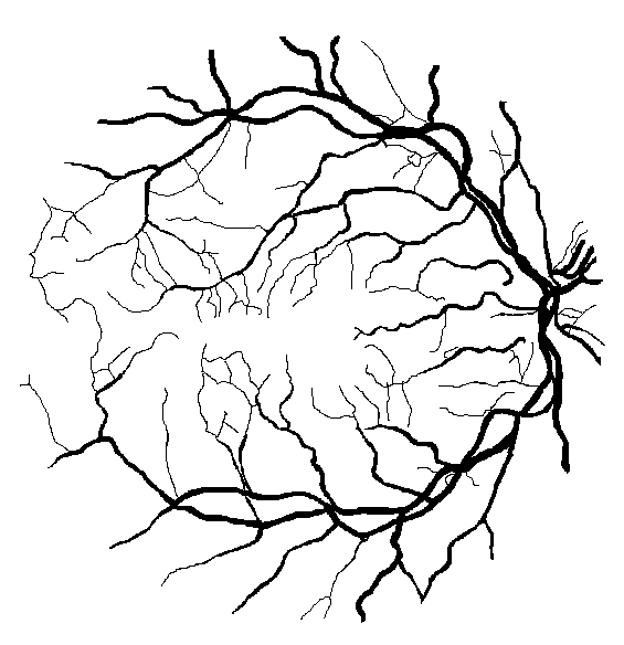
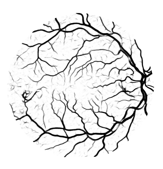
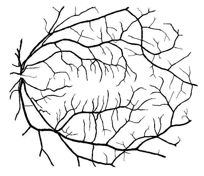
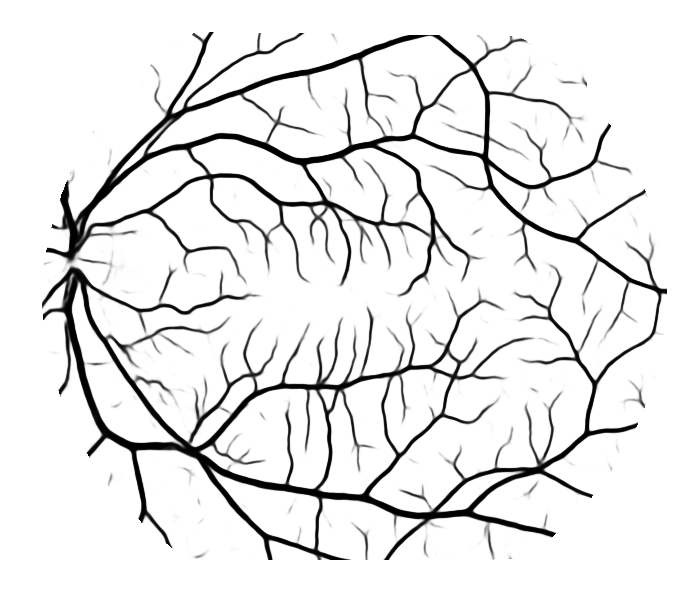
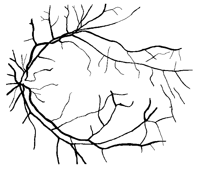
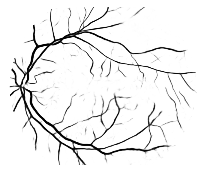
Figure 10: Examples of segmentation by non-SP (left) and SP (middle) models for images (right) of DRIVE (a) and STARE (b, c) database. Red pixels: FP errors, blue: FN errors, black: TP, white: TN.
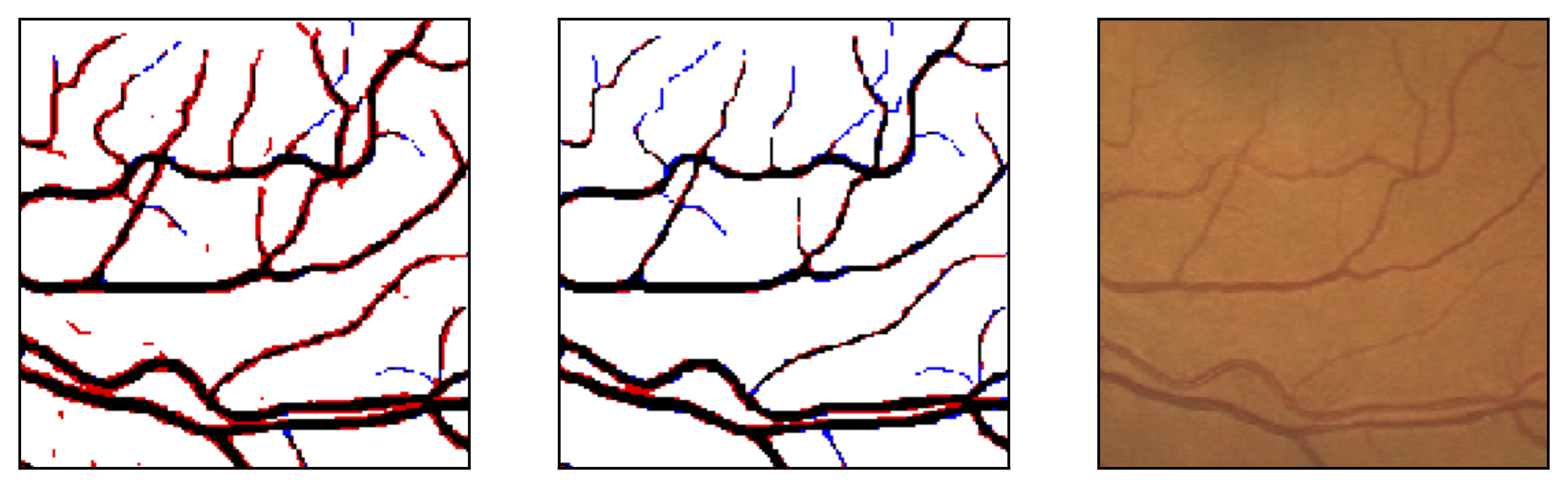
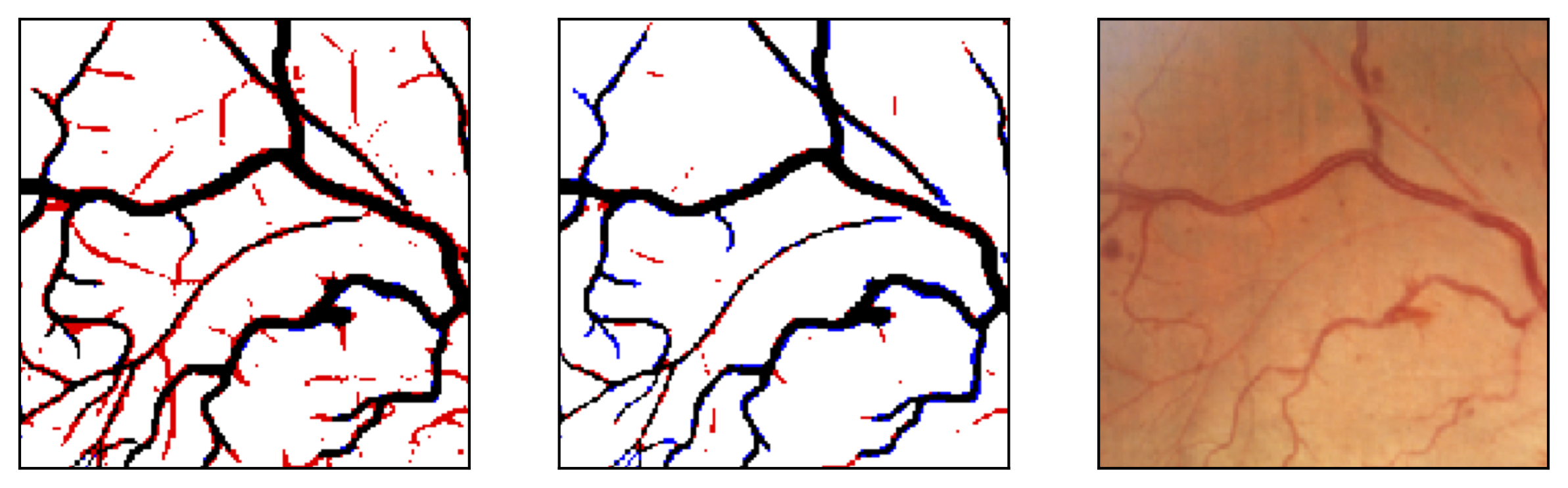
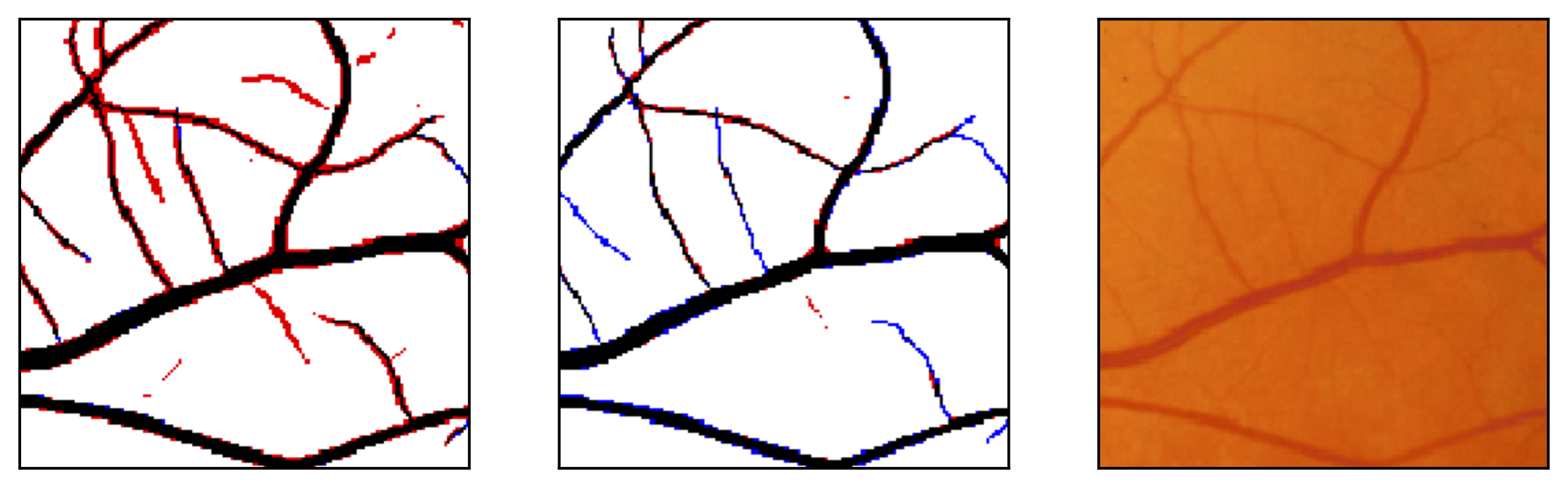
Figure 11: Image fragments with central vessel reflex (a) and corresponding segmentation results (b); CHASE database.
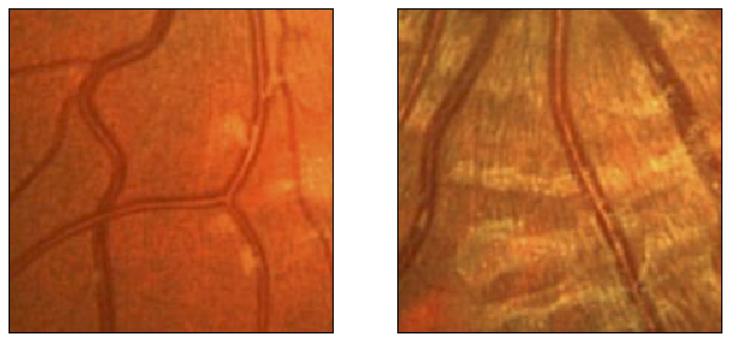
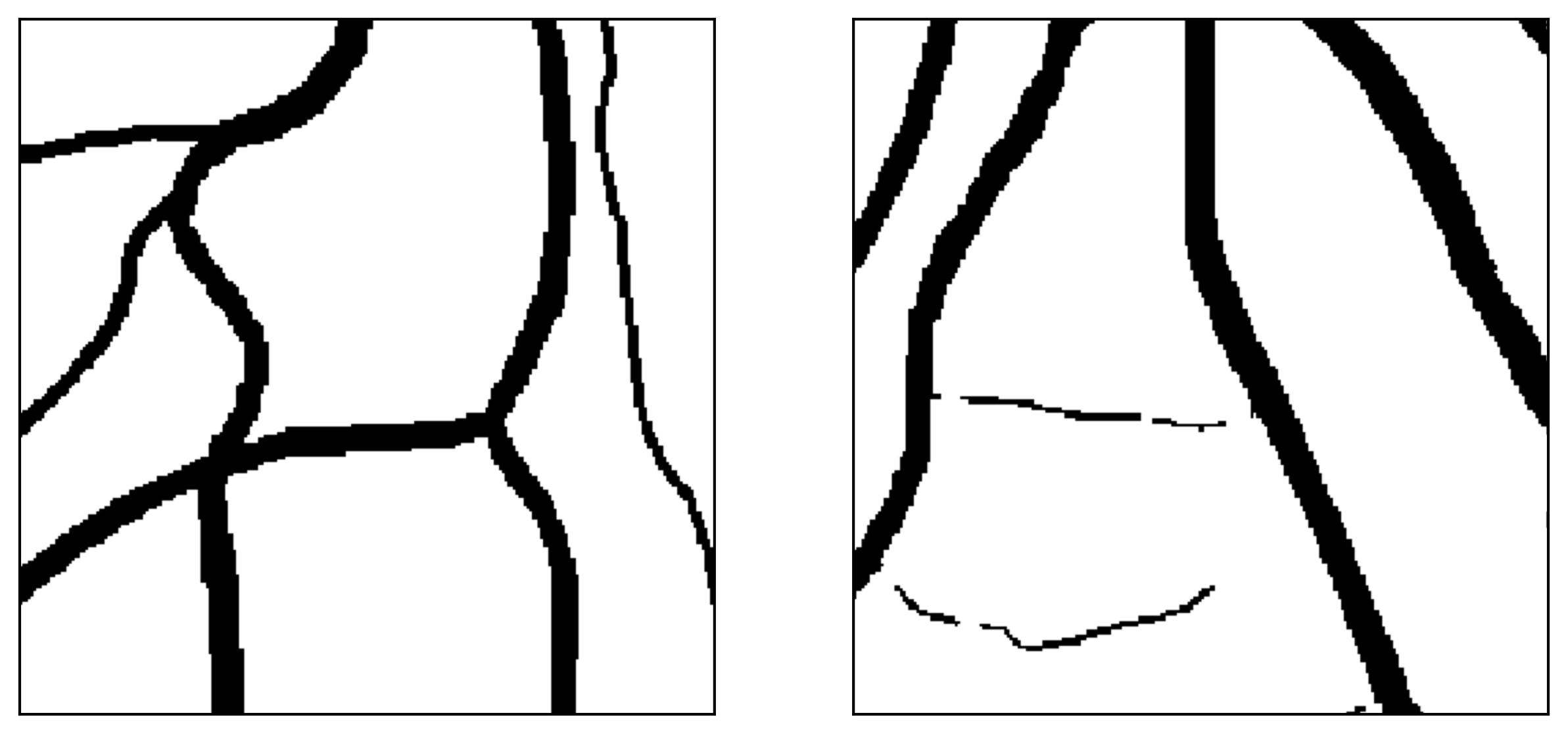
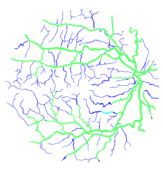
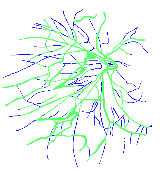
Figure 12: Two manual segmentations from the DRIVE database (images #22 and #34) automatically partitioned into thick vessels (green) and capillaries (blue).